R数据可视化|使用Scatterplot3d包制作3D散点图
介绍
R 中有许多包(RGL、car、lattice、scatterplot3d等)用于创建3D 图形。
本教程介绍了如何使用 R 的 scatterplot3d包 在 3D 空间中生成散点图。
scaterplot3d 使用起来非常简单,可以通过在已经生成的图形中添加补充点或回归平面来轻松扩展。
它可以很容易地安装,因为它只需要一个已安装的 R 版本。
安装并加载 scaterplot3d
1 | install.packages("scatterplot3d") |
准备数据
iris 数据集将被使用进行画图:
1 | data(iris) |
Iris 也称鸢尾花卉数据集,是一类多重变量分析的数据集。
数据集包含150个数据样本,分为3类,每类50个数据,每个数据包含4个属性。
可通过花萼长度,花萼宽度,花瓣长度,花瓣宽度4个属性预测鸢尾花卉属于(Setosa,Versicolour,Virginica)三个种类中的哪一类。
函数 scatterplot3d()
一个简化的格式是:
1 | scatterplot3d(x, y=NULL, z=NULL) |
x, y, z 是要绘制的点的坐标。参数 y 和 z 可以是可选的,具体取决于 x 的结构。
那么在什么情况下,y 和 z 是可选变量?
情况1: x是 zvar ~ xvar + yvar 类型的公式。xvar、yvar 和 zvar 用作 x、y 和 z 变量
情况2: x是一个矩阵,包含至少3列,分别对应于x、y和z变量
基本 3D 散点图
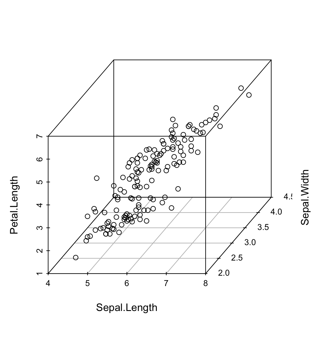
1 | scatterplot3d(iris[,1:3]) |
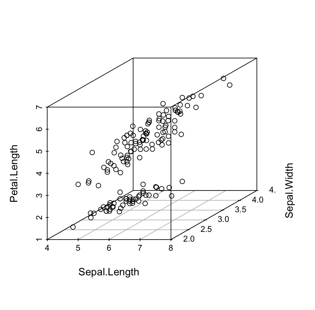
1 | # 改变点视图的角度 |
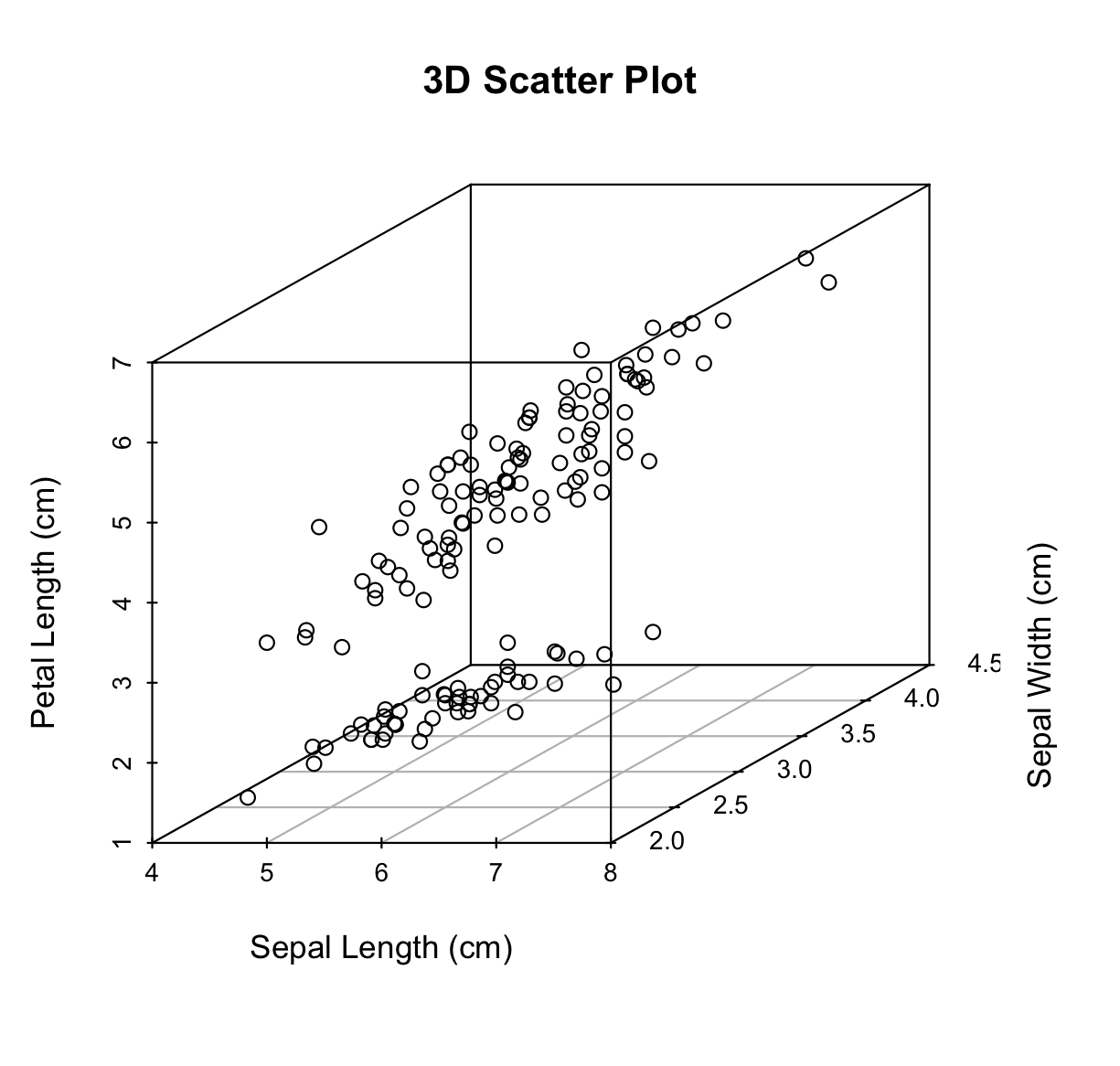
更改主标题和轴标签
1 | scatterplot3d(iris[,1:3], |
改变点的形状和颜色
可以使用参数 pch 和 color:
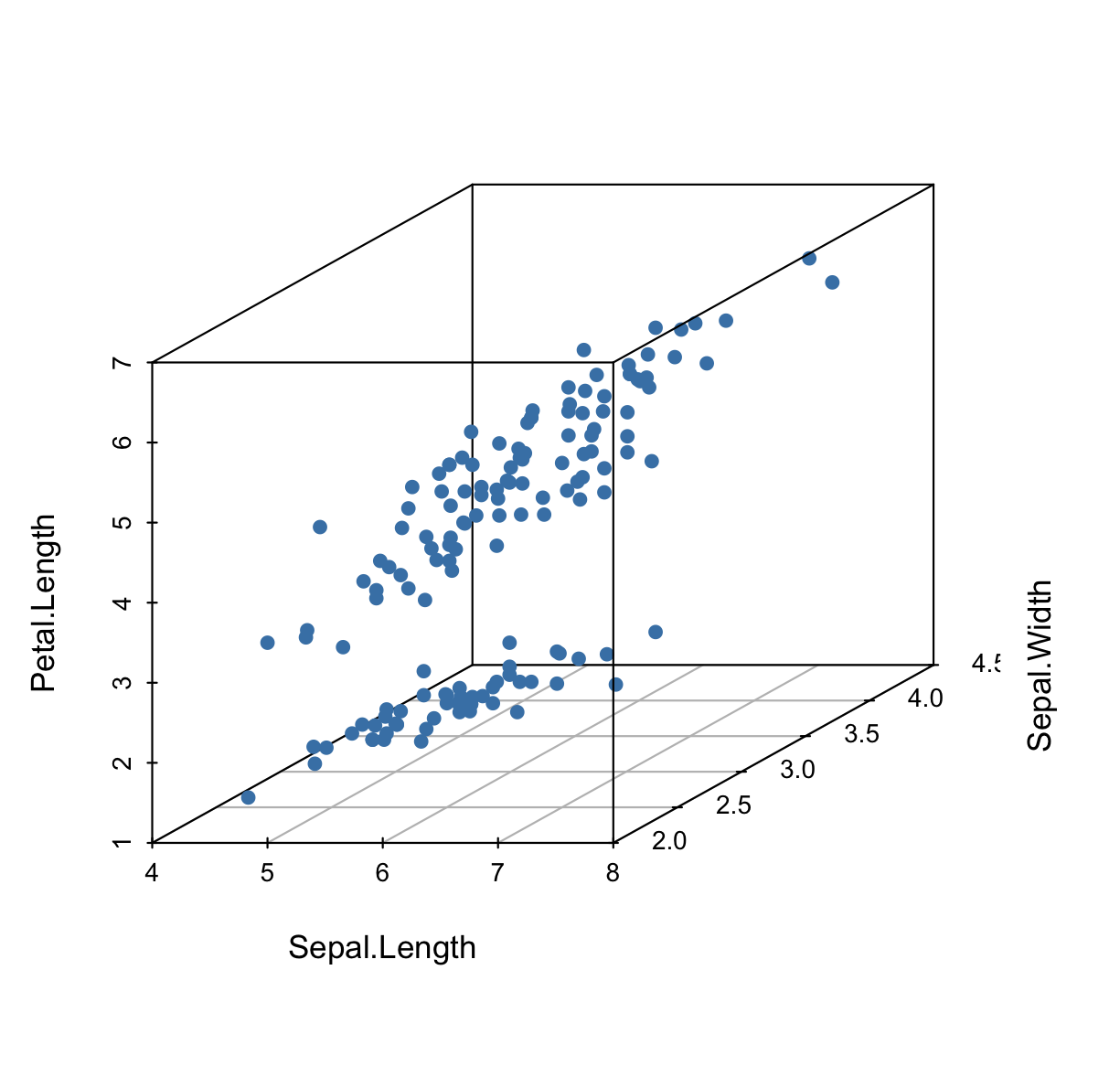
1 | scatterplot3d(iris[,1:3], pch = 16, color="steelblue") |
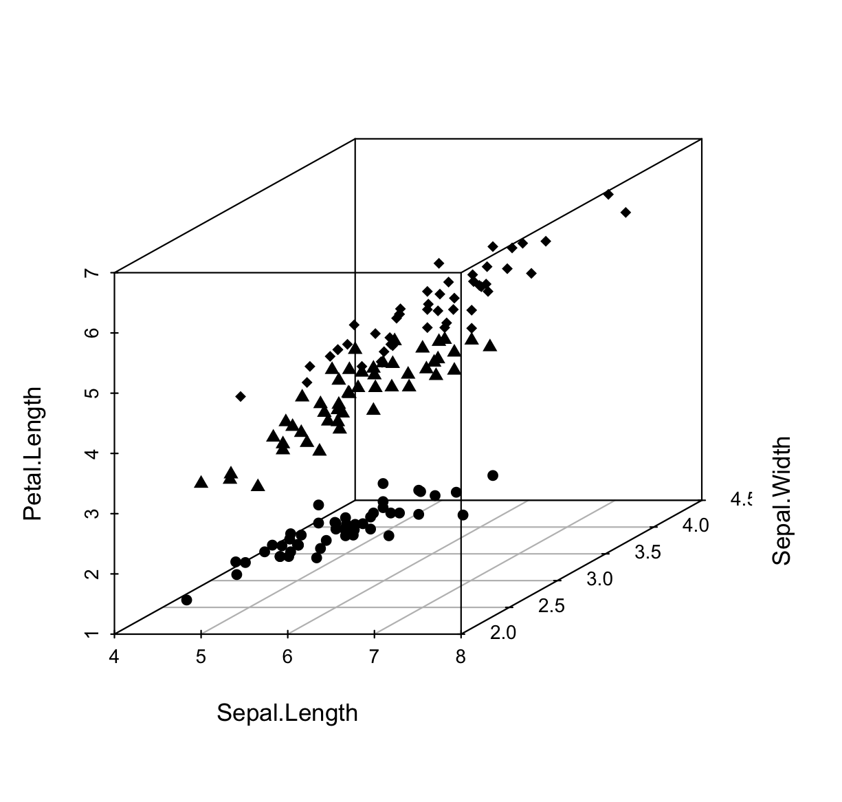
按组更改点形状
1 | shapes = c(16, 17, 18) |
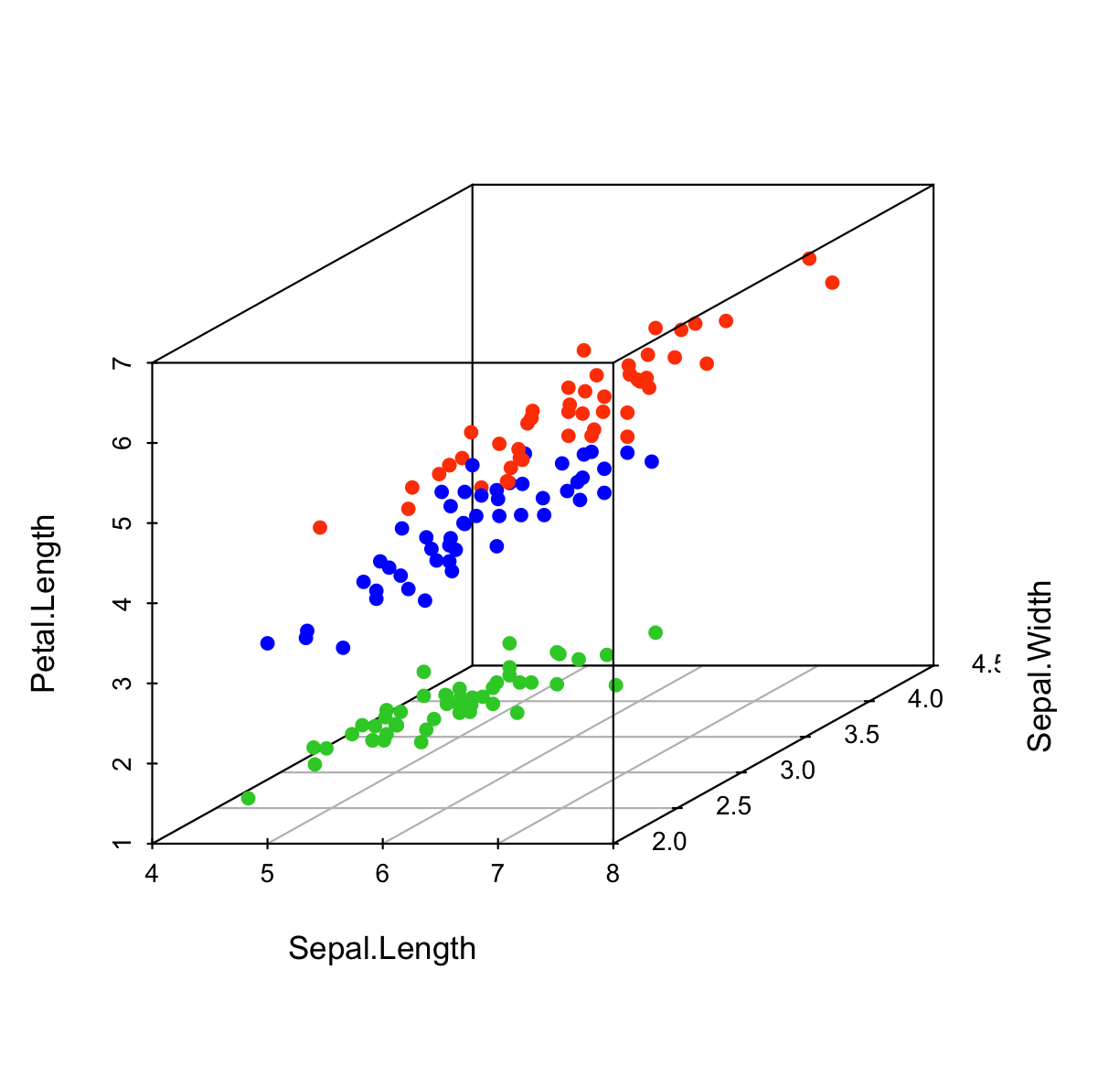
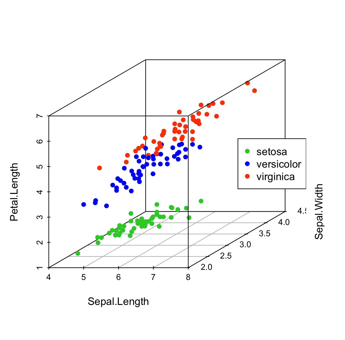
按组更改点颜色
1 | colors <- c("#32CD32", "#0000FF", "#FF4500") |
更改图形的全局外观
可以使用以下参数:
- grid : 一个逻辑值。如果为 TRUE,则在底部绘制网格。
- box : 一个逻辑值。如果为 TRUE,则在图片上方周围绘制一个框
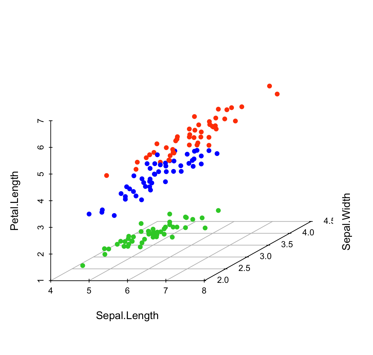
删除周围的框
1 | scatterplot3d(iris[,1:3], pch = 16, color = colors, |
- x、y 和 z 是指定点的 x、y、z 坐标的数值向量。
x 可以是一个矩阵或一个包含 3 列对应于 x、y 和 z 坐标的数据框。
在这种情况下,参数 y 和 z 是可选的- grid 指定绘制网格的面。
可能的值是“xy”、“xz”或“yz”的组合。 示例:grid = c(“xy”, “yz”)。
默认值为 TRUE 以仅在 xy 平面上添加网格。- col.grid, lty.grid: 用于网格的颜色和线型
在 scatterplot3d 图形的不同面上添加网格:
1 | # 1. 源函数 |
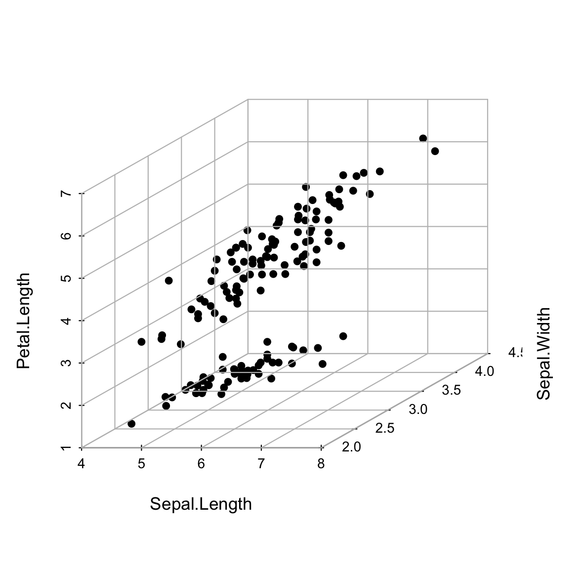
上图中有一个问题就是网格是在点上绘制的。
在下面的R代码中,我们将使用以下步骤将点放在前景中:
- 创建空的 scatterplot3 图形,并将 scatterplot3d() 的结果指定给 s3d
- 函数 addgrids3d() 用于添加网格
- 最后,函数 s3d$points3d 用于在三维散点图上添加点
1 | # 1. 源函数 |
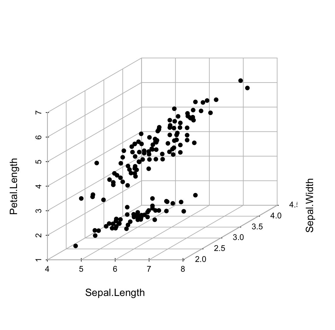
函数 points3d() 将在下一节中描述。
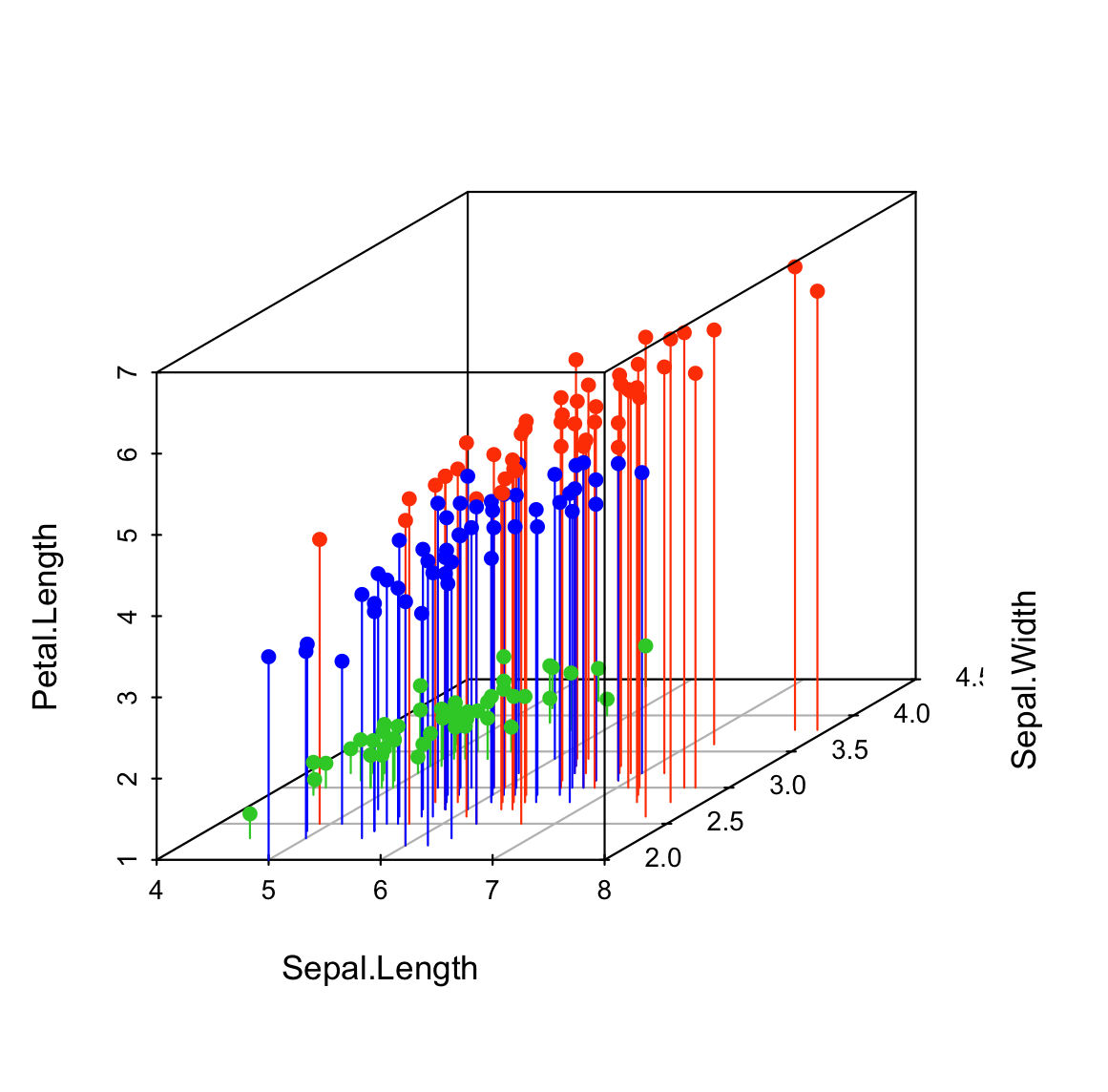
添加 bars
使用参数 type=“h”。这有助于非常清楚地查看点在 x-y 上的位置。
1 | scatterplot3d(iris[,1:3], pch = 16, type="h", |
修改 scatterplot3d 输出
scatterplot3d 返回一个函数闭包列表,可用于在现有绘图上添加元素。
返回的函数是:
- xyz.convert(): 将 3D 坐标转换为现有 scatterplot3d 的 2D 平行投影。 它可用于向绘图中添加任意元素,例如图例。
- points3d():在现有图中添加点或线
- plane3d():将平面添加到现有绘图中
- box3d():在图周围添加一个框
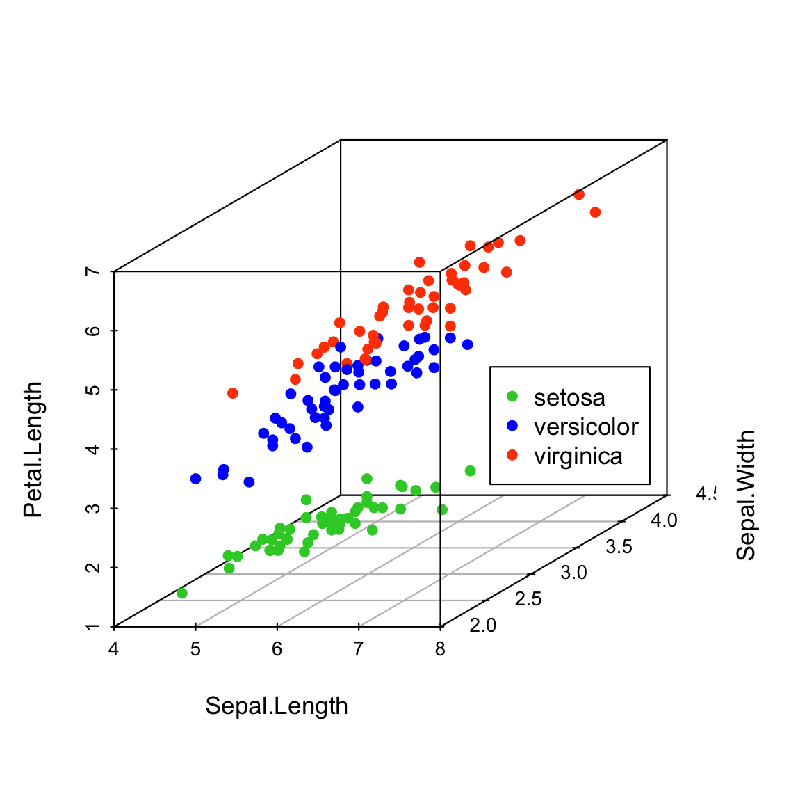
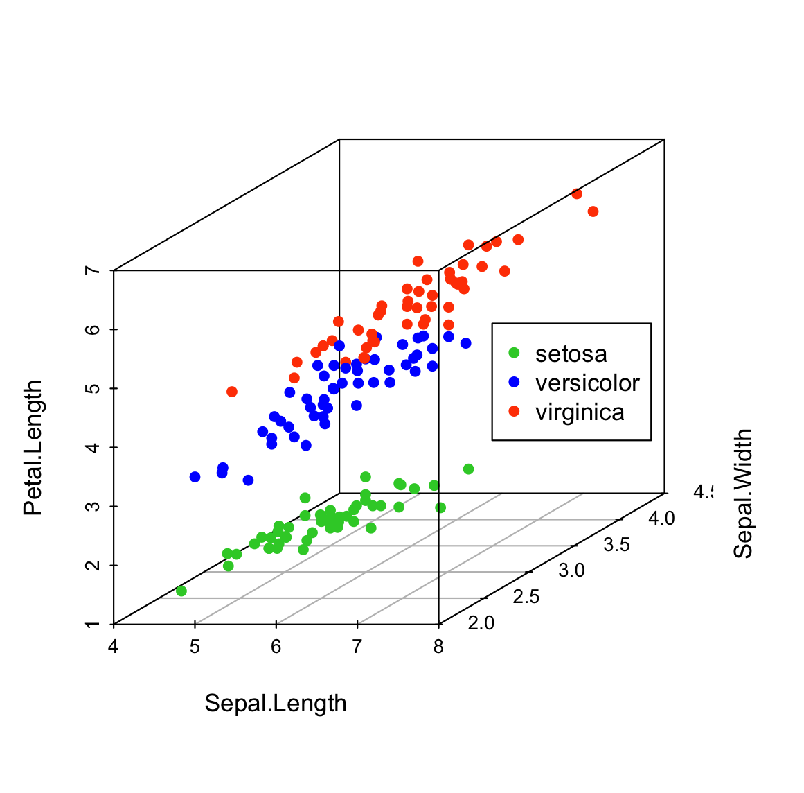
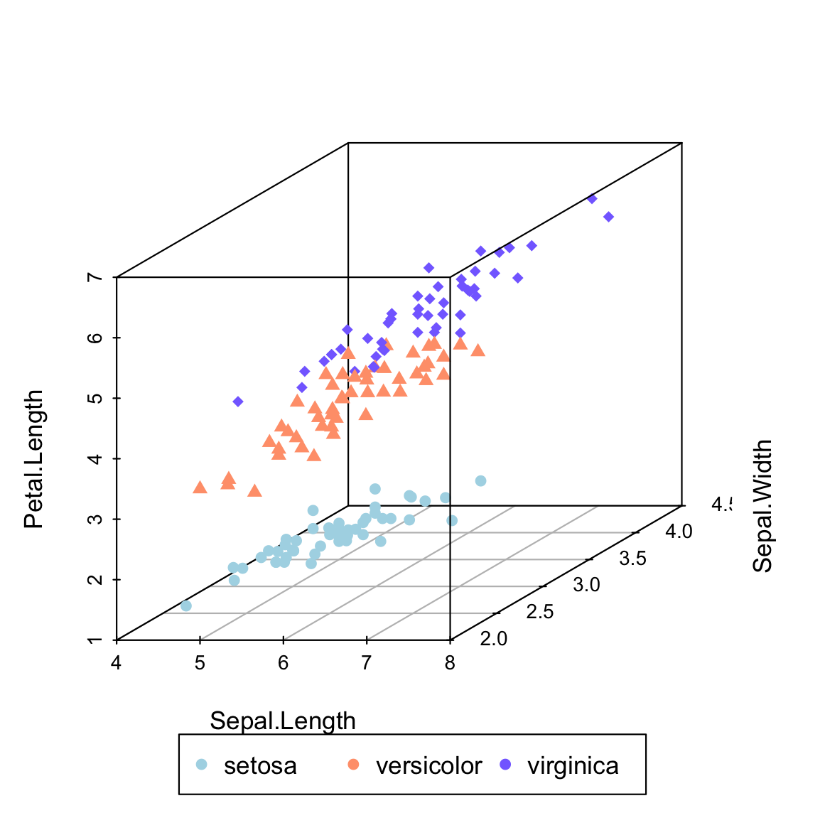
添加图例
使用 xyz.convert() 指定图例位置
- 将 scatterplot3d() 的结果指定给 s3d
- 函数 s3d$xyz.convert() 用于指定图例的坐标
- 函数 legend() 用于添加图例
1 | s3d <- scatterplot3d(iris[,1:3], pch = 16, color=colors) |
也可以使用以下关键字指定图例的位置:“bottomright”、“bottom”、“bottomleft”、“left”、“topleft”、“top”、“topright”、“right”和“center”
使用关键字指定图例位置
1 | # 图例位置修改为 "right" |
1 | # 使用参数 inset,其中inset设置值越大,图例越向左偏移 |
1 | # 图例位置修改为 "bottom" |
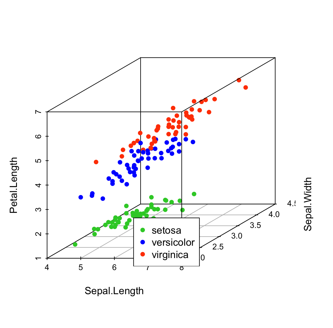
使用关键字来指定图例位置非常简单。但是,有时,某些点和图例框之间或轴和图例框之间存在重叠。
那么有什么解决方案可以避免这种重叠吗?
当然,对于函数 Legend(),有多种使用以下参数组合的解决方案:
- bty = “n” :删除图例周围的框。 在这种情况下,图例的背景颜色变得透明,重叠点变得可见
- bg = “transparent” :将图例框的背景颜色更改为透明颜色(仅当 bty != “n” 时才有可能)
- inset :修改图边距和图例框之间的距离
- horiz :一个逻辑值; 如果为 TRUE,则水平而不是垂直设置图例
- xpd :逻辑值; 如果为 TRUE,则它允许将图例项绘制在绘图之外
自定义图例位置
1 | # 自定义点形状 |
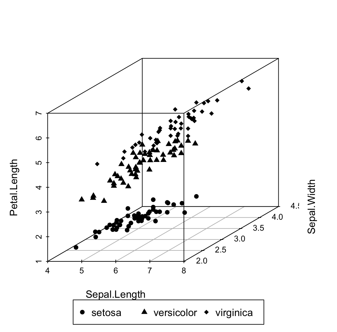
1 | # 自定义颜色 |
在上面的 R 代码中,可以使用参数 inset、xpd 和 horiz 来查看对图例框外观的影响。
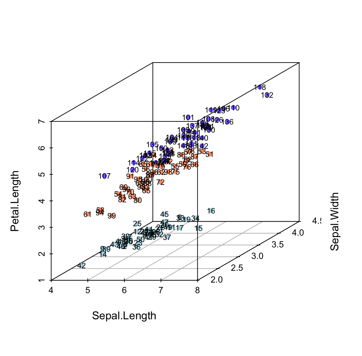
添加点标签
函数 text() 的用法如下:
1 | scatterplot3d(iris[,1:3], pch = 16, color=colors) |
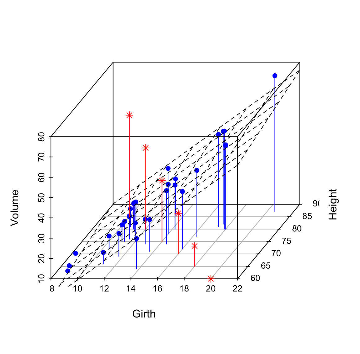
添加回归平面和补充点
- 将 scatterplot3d() 的结果赋值给 s3d
- 线性模型计算如下:lm(zvar ~ xvar + yvar)。 假设:zvar 取决于 xvar 和 yvar
- 函数 s3d$plane3d() 用于添加回归平面
- 使用函数 s3d$points3d() 添加补充点
将使用数据集:
1 | data(trees) |
带有回归平面的 3D 散点图:
1 | # 3D scatter plot |
 微信
微信 支付宝
支付宝